How to Create Sparklines in Excel

How to Create Sparklines in Excel

When working with data in Excel, you will sometimes want to create a sparklines to view a mini Sparkline within a single cell near your sourece data. Sparklines are a nice tool to provide quick snapshots of data trends without creating a Sparkline or graph in Excel.

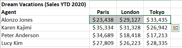
Step 1: Select the data you want in the Sparkline

Use your mouse to select the data you would like to include in your sparkline.

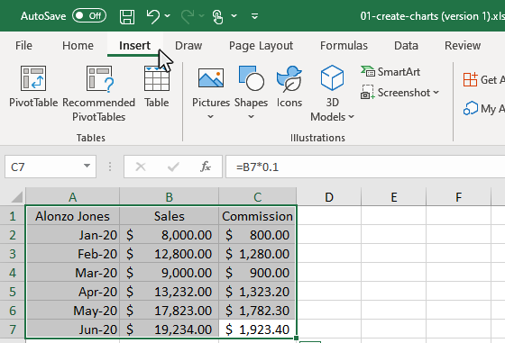
Step 2: Click the Insert Tab

Once the data is selected, click in the Insert tab to display the Sparkline options on the ribbon.

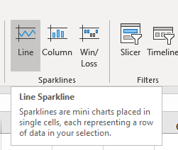
Step 3: Click on one of the Sparkline types

In the Sparkline section of the Insert tab, click on one of the Sparkline types displayed.

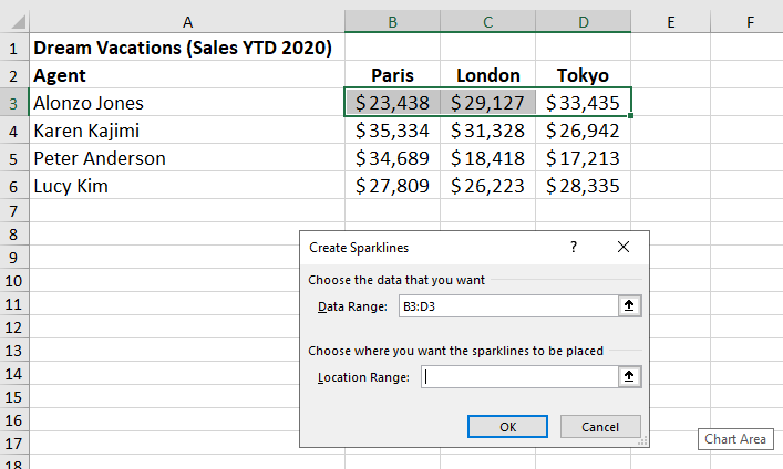
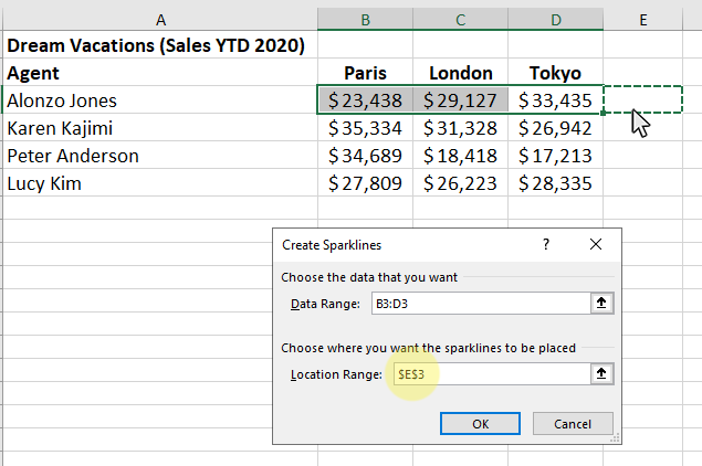
Step 4: Select the Cell for the Sparkline to appear

After you select the sparkline type, a window will appear and ask you for the location where the sparkline should be placed. Click your mouse inside the box for Location Range, and then click the cell where you want the sparkline to appear. The cell reference for the selected cell will appear in the Location Range box.

The cell reference for the selected cell will appear in the Location Range box.

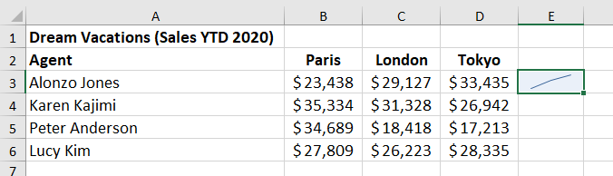
Step 5: Click OK, and the sparkline will appear in the selected cell

After you have selected the cell location for the sparkline, just click ok and the sparkline will appear.

Topic #13

How to Create Sparklines in Excel

Thanks for checking out this tutorial. If you need additional help, you can check out some of our other free Excel Chart Tutorials, or consider taking an Excel class with one of our professional trainers.