How to Move and Resize Charts in Excel

How to Move and Resize Charts in Excel

After creating your chart in Excel, you may want to change the size of the chart, move it to a different spot on the worksheet, or move it to a different worksheet. This tutorial will teach you how to move and resize charts and graphs in Excel.

How to Move a Chart in Excel

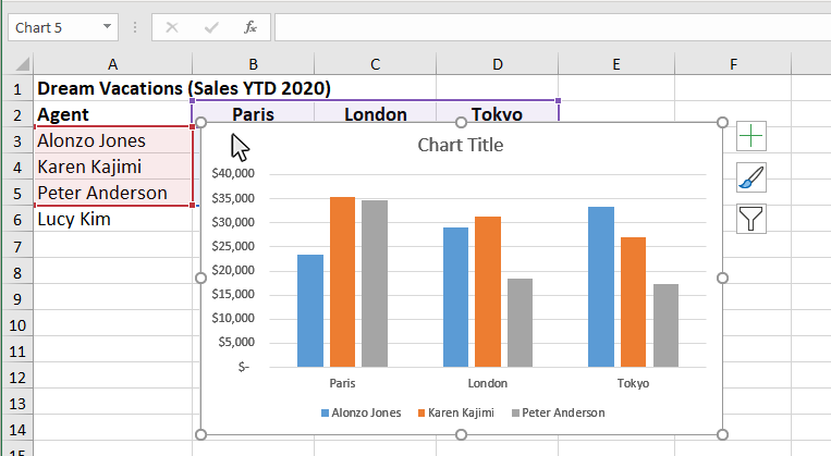
Step 1: Click on a blank area of the chart

Use the cursor to click on a blank area on your chart. Make sure to click on a blank area in the chart. The border around the entire chart will become highlighted. Once you see the border appear around the chart, then you know it is ready to be moved.

Step 2: Move the chart to the desired location

You can use your mouse to drag the selected chart to the location you want on the spreadsheet. Once you have placed the chart in the correct location, click a blank cell in the spreadsheet and the chart will be de-selected.

Alternate Method: An alternate method for moving the chart to a specific location is to use the arrow keys on your keyboard to move and reposition the chart.

How to Resize a Chart In Excel

Step 1: Click on a blank area of the chart

Select the chart you want to resize, and make sure the circular move handles appear on the border around the chart.

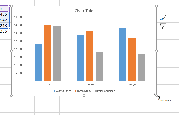
Step 2: Use the Move handles to resize the chart

The circular move handles on the border of the chart allow you to resize the entire chart, or to make horizontal and vertical changes to the size of the chart. To change the size of the whole chart, mouse over one of the move handles on the corner of the chart and drag it out to make it larger, or drag it in to make it smaller. When you see the mouse pointer change to the double arrow

Top make horizonal or vertical changes to the chart size, use the move handles on the top, bottom or sides of the chart to make the appropriate changes.

How to Move a Chart to a New Worksheet in Excel

Sometimes, you will not want to display your chart on the same worksheet as the chart's source data and have it display on its own tab. To do this, complete the following steps:

Step 1: Click on a blank area of the chart

Use the cursor to click on a blank area on your chart. Make sure to click on a blank area in the chart. The border around the entire chart will become highlighted. Once you see the border appear around the chart, then you know it is ready to be changed.

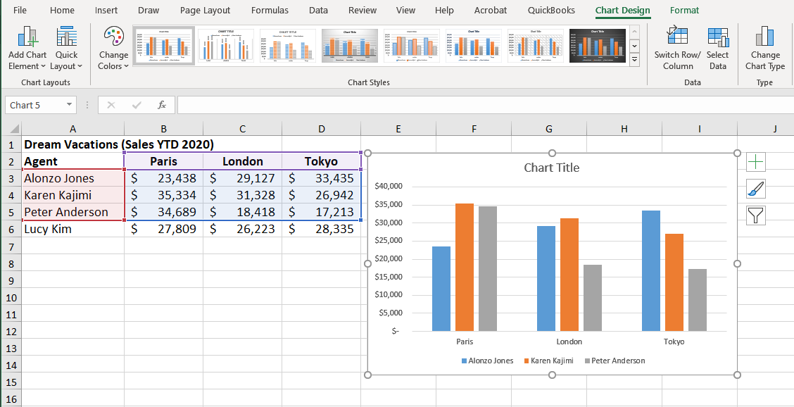
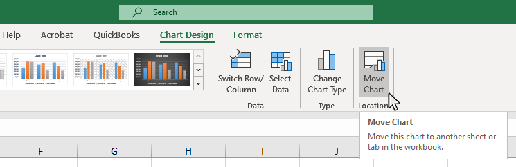
Step 2: Select the Chart Design tab

After you have selected your chart, the Chart Design tab will appear on the ribbon. This tab will only appear when a chart is selected. Options included in this tab are Chart Layouts, Chart Styles, Data, Type and Location.

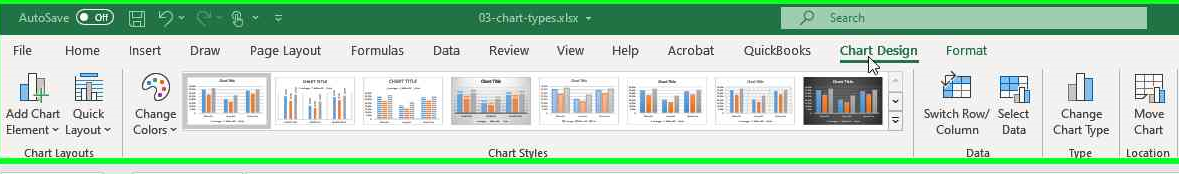
Step 3: Click the Move Chart Button

The Move Chart button is in the Location section of the Chart Design tab. Click on the Move Chart button and a pop-up menu will appear with all the Move Chart options available.

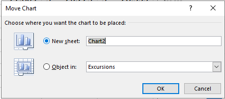
Step 4: Select the New Sheet Option on the Move Chart pop-up window

The final step is to select the New Sheet option on the Move Chart pop-up window. Once you select this option and hit OK the chart will appear on its own worksheet and no longer display on the original sheet. Changes to the chart data will still effect the appearance of the chart even if they are not on the same page.

Topic #4

How to Change the Chart Style in Excel

Thanks for checking out this tutorial. If you need additional help, you can check out some of our other free Excel formatting tutorials, or consider taking an Excel class with one of our professional trainers.