How to Make a Chart or Graph in Excel

How to Make a Chart or Graph in Excel

When working in an Excel spreadsheet, you may want to display specific data from your worksheet in a visual format called a Chart or Graph. Excel provides a number of options to visually represent your data in useful ways. This tutorial will teach you how to create a basic chart in Excel. Subsequent tutorials will cover all of the different tools and features available for customizing your charts and graphs.

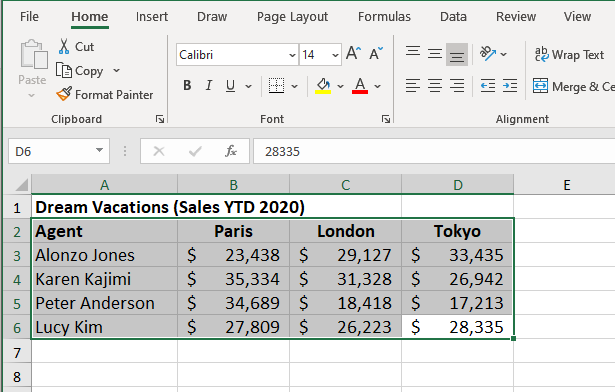
Step 1: Select the Data to use in your Chart

The first step when building any chart is to select the data to use in the chart or graph. Use the cursor to highlight the cells that contain the data you want to include in your chart. The cells that are selected will be highlighted with a green border.

Step 2: Select Your Chart Type

Once, you have selected your data, click the Insert tab and then click the Recommended Charts Button in the Charts Group on the ribbon. You will see a variety of chart types to choose from. Clicl OK and the chart will appear in the workbook.

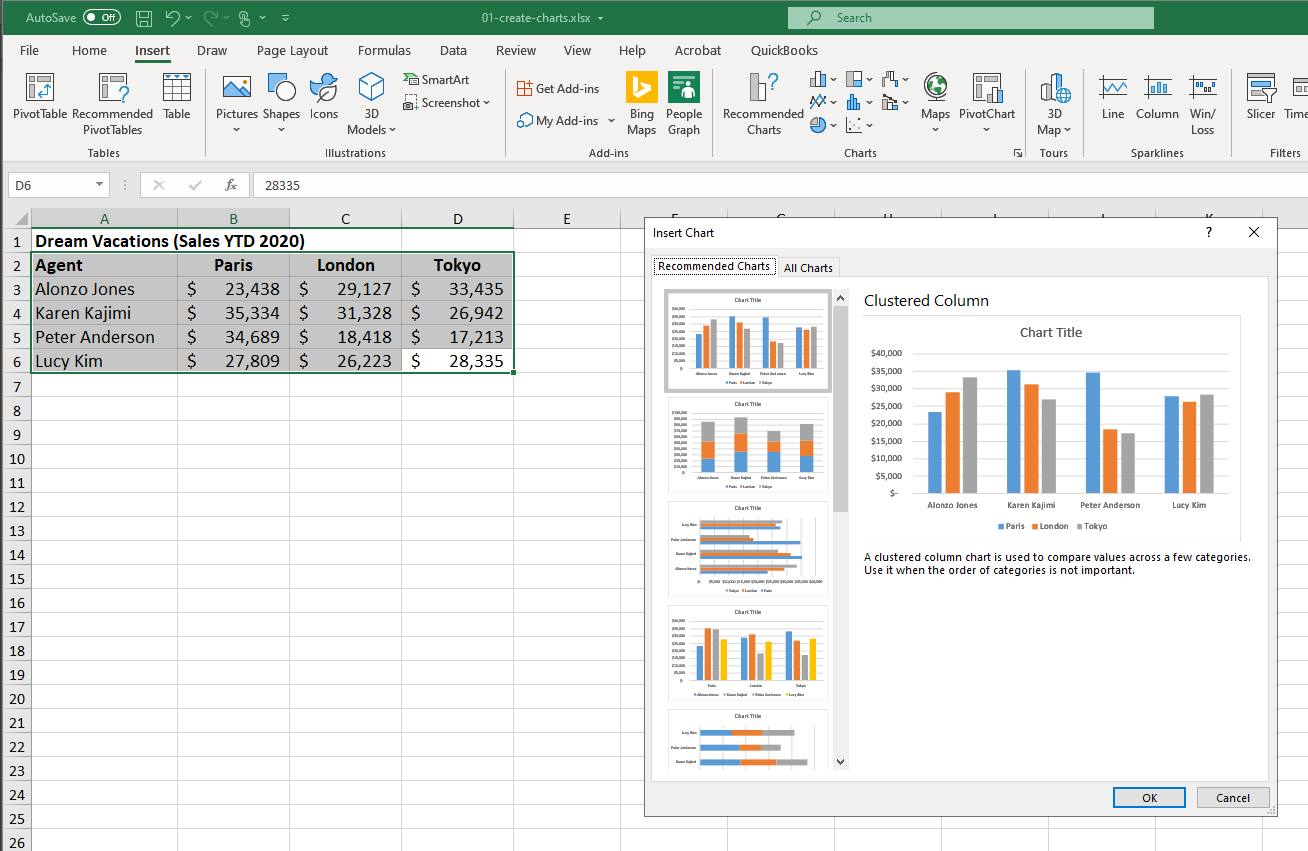
In the Charts Group on the ribbon there are also shortcuts to the most poplular chart types. You can also use these buttons to change the chart type at any time.

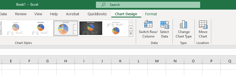
Step 3: Edit your Chart Design

Now that you have created your chart and selected your chart type, you can use the Chart Design tab to modify items like your Chart Design, Data, Chart Type and chart location. The Chart Design menu only appears when you click on the chart or graph you created.

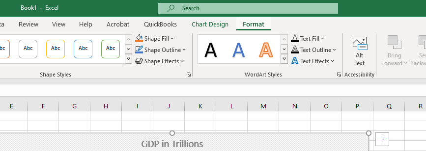
Step 4: Edit your Chart Formatting

The second tab that appears when you click on your chart is the Format tab. The Format tab allows Excel users to customize the appearance of their charts in a variety of ways. You can select different parts of the chart for editing by using the Current Selection dropdown menu. Additional features include Inserting shapes, Sharp Styles, WordArt Styles, Accesibility settings and options to change the Size and Position of the chart and objects within it.

Topic #2

How to Change the Chart Type in Excel

Thanks for checking out this tutorial. If you need additional help, you can check out some of our other free Excel formatting tutorials, or consider taking an Excel class with one of our professional trainers.