The Box and Whisker chart is the third statistical chart included in the chart toolbox starting with Google Sheets 2016. The other two, Histogram and Pareto charts, have their own tutorial. The box and whisker chart graphically depicts numerical data through their statistical quartiles (minimum, first quartile, median, third quartile and maximum).

The box shows the value of the first quartile at the bottom of the box, the value of the third quartile at the top of the box type of chart and the median value inside the box. The whiskers are lines that extend from the boxes to the minimum and maximum values. An outlier is a value that falls outside the expected range of values; they usually appear as a singular dot on the chart.

This tutorial will show you how to make and edit a Box and Whisker Chart in Google Sheets

How to Make a Box and Whisker chart in Google Sheets

Step 1: Select the data you want displayed in the Box and Whisker chart

Use your mouse to select the data you want included (holding down the control key allows non-contiguous ranges of data to be selected. If the data set is extremely large it may be easier if columns or rows are hidden).

Step 2: Click the Insert Tab, and then Click Insert Statistic Chart in the Charts Group.

After selecting the data for the chart, click on the Insert tab and select Insert Statistic Chart choice from the charts group.

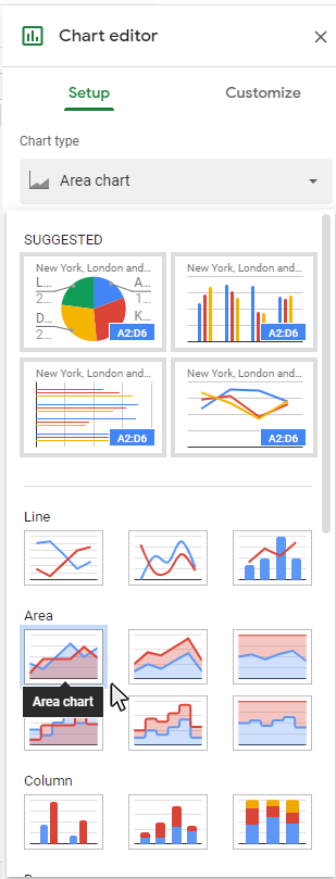
Step 3: Select the Box and Whisker chart type.

Click the Box and Whisker button from the Statistical Chart window, then the chart will appear in the workbook.

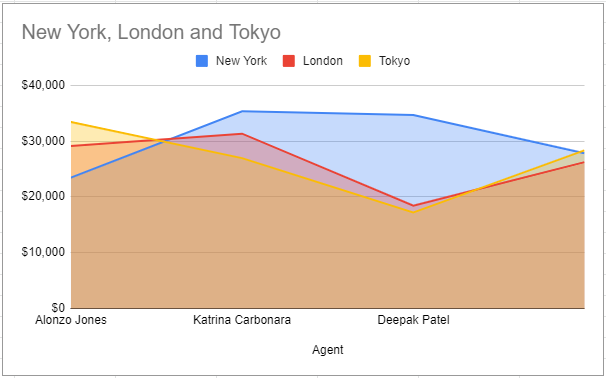
Result: Your Box and Whisker Chart will appear on your worksheet

YYou will now see your Box and Whisker chart appear in your worksheet. Now you can start changing chart elements and formatting of your chart. Google Sheets will do many things automatically, for example gap width, Show outlier points and Quartile Calculation. Continue reading for more details on modifying chart elements and chart formatting.

---

How to Add Chart Elements to a Box and Whisker chart in Google Sheets

Step 1: Click on a blank area of the chart

Use the cursor to click on a blank area on your chart. Make sure to click on a blank area in the chart. The border around the entire chart will become highlighted. Once you see the border appear around the chart, then you know the chart editing features are enabled.

Step 2: Click on the Chart Elements button next to the chart

Once the chart name area is highlighted, you will see the Chart Elements button next to upper right-hand side of the chart. The button looks like a plus sign. Doing this will open the Chart Elements window.

Step 3: Check the Chart Elements you would like to add from the Chart Elements window

Once you have opened the Chart Elements window, you will see a number of items you can select to add to your chart. Check the Chart Elements you would like to display and they will appear on your chart. You can click on the arrow next to each Chart Element option for some additional formatting options.

Here are the available chart elements for a Box and Whisker Chart:

• Axes
• Axes Titles
• Chart Title
• Data Labels
• Data Table
• Gridlines
• Legend

Each of these chart elements can be formatted in a variety of ways. Please see our other tutorials on how to add and format each chart element.

How to Format a Box and Whisker chart in Google Sheets

Step 1: Right-Click on a blank area of the chart

Use the mouse to right-click on a blank area on your chart. On the menu that appears select the Format Chart Area option.

Step 2: Select the Format Chart Area option

On the menu that appears select the Format Chart Area option. Doing this will open the Format Chart Area panel on the right side of the workbook.

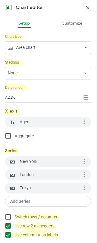
Step 3: Use the Format Chart Area panel to make changes to the appearance of your chart

Once you have opened the Format Chart Area panel, you will see a number of items you can modify on your chart. use these features to create a custom look for your Box and Whisker chart.

Here are the available chart elements for a Box and Whisker Chart:

• Fill
• Border
• Shadow
• Reflection
• Glow
• Soft Edges
• 3-D Format
• Size
• Properties

Please note: You can also right click on any of your chart elements and open a separate formatting panel for that particular item. The Format Chart Area panel will be the one you want to use when formatting the main structure of the chart.

How to Modify the Organization of a Box and Whisker chart in Google Sheets

Step 1: Right-Click on any of the Boxes of the chart

Use the mouse to right-click on any of the Boxes on your chart.

On the menu that appears select the Format Data Series.

Step 2: Select the Format Axis option

On the menu that appears select the Format Axis option. Doing this will open the Format Data Series panel on the right side of the workbook.

Topic #13

How to Make a Waterfall Chart in Google Sheets

Thanks for checking out this tutorial. If you need additional help, you can check out some of our other free Google Sheets Chart tutorials, or consider taking an Google Sheets training class with one of our professional trainers.