How to Use Conditional Formatting in Excel

How to Use Conditional Formatting in Excel

This tutorial on how to Use Conditional Formatting in Microsoft Excel may be of interest to you if you want to visually highlight data that meets certain conditions in your Excel workbooks. Conditional Formatting is a very useful tool that helps users to pinpoint data that is important to them or their audience. Typically this feature is used to highlight strong and weak results, outlier data and to identfy trends in your datasets.

Conditional Formatting is a relatively simple process and is available across all versions of Excel.

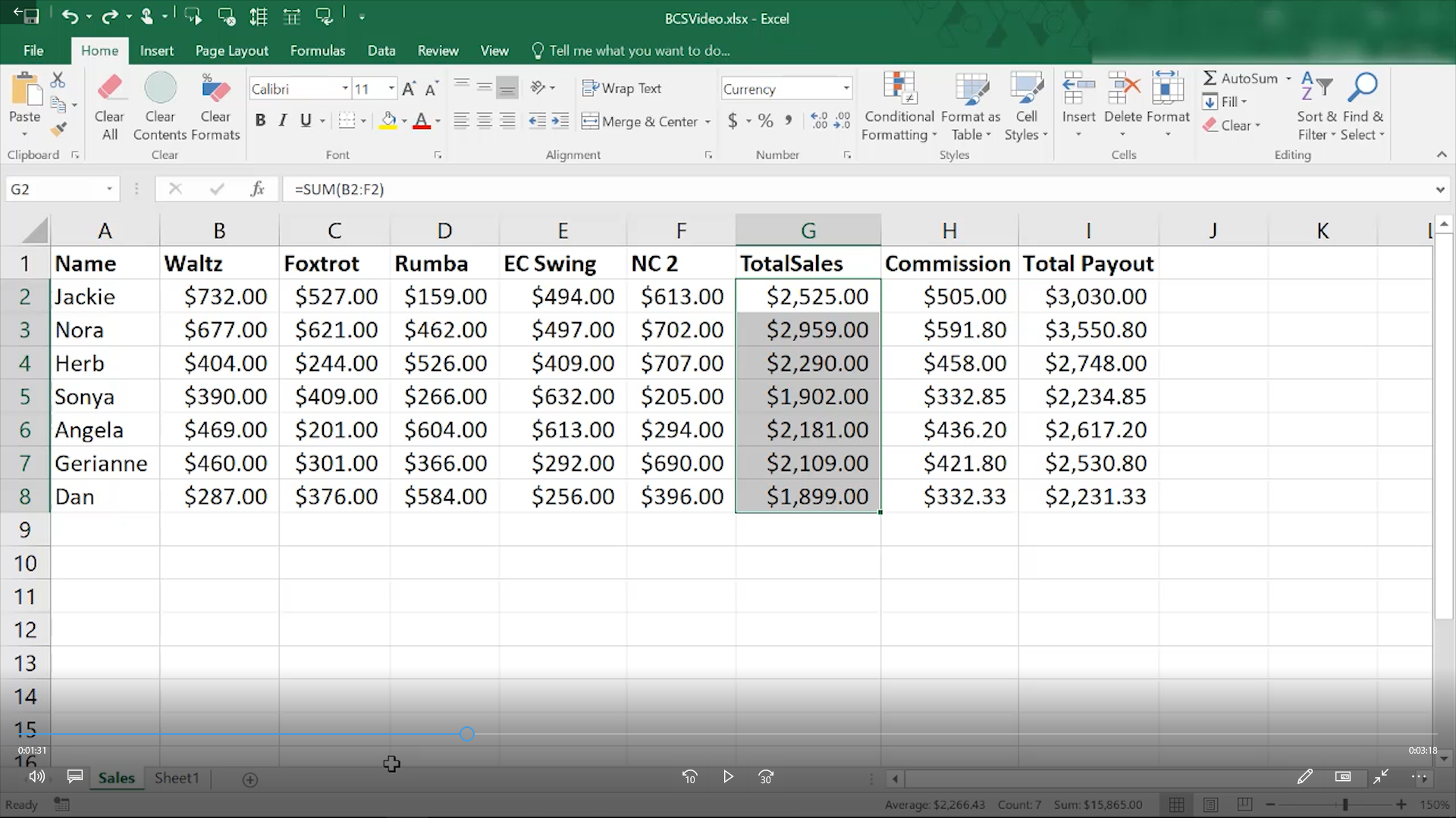
Step 1: Select the Cells You Want to Format

Use the cursor to highlight the cells you want to apply conditional formatting to. The cells that are selected will be highlighted with a green border.

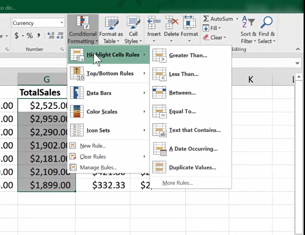
Step 2: Determine the Rules You Want to Apply to the Cells

To find the Conditional Formatting button, open the Home tab and look in the Styles Section. Click the Conditional Formatting Button and you will see a dropdown menu. The dropdown menu contains a number of preformatted rule groups that you can choose from.The rule group options to choose from include Highlight Cells, Top/Bottom Rules, Data Bars, Color Scales and Icon Sets.

Once you select the rule group you want, a secondary dropdown menu will appear where you can select the specific rule you want to apply. There are also options for creating custom conditional formatting rules.

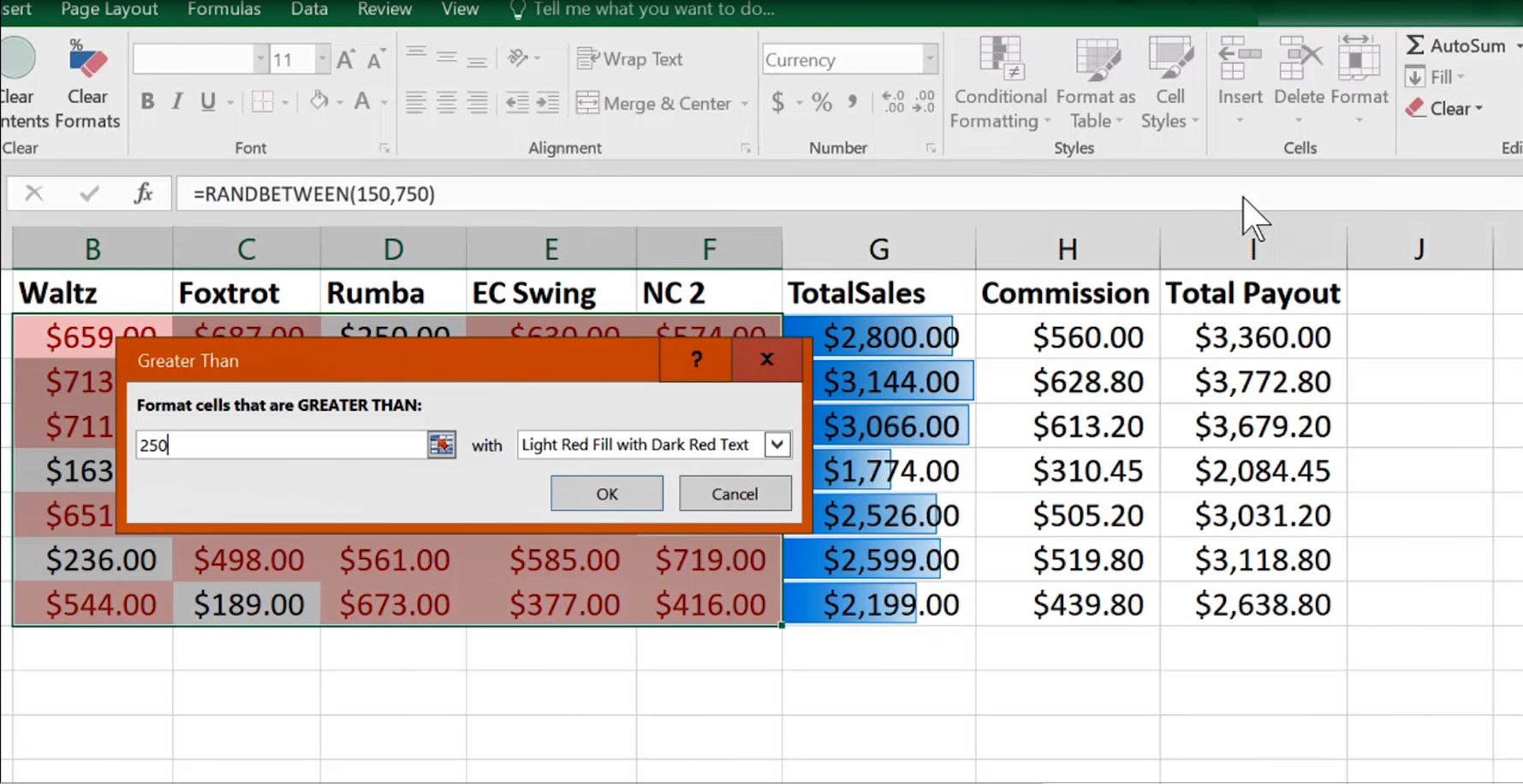
Step 3: Determine the Formatting You Want to Apply to the Cells

Now that you have selected a rule, in most cases, you will see a dialog box appear. In the dialog box you will be able to set the specific conditions for your rule to be valid. You will also be able to select the specific formatting you want applied when the rule is true.

You are able to apply multiple rules to a cell, and the Conditional formatting is dynamic, so you fomatting can update when the cell values change.

Related tutorials

• How To Lock Cells in Excel
• How To Merge Cells in Excel
• How To Unmerge Cells in Excel

Thanks for checking out this tutorial. If you need additional help, you can check out some of our other free Excel formatting tutorials, or consider taking an Excel class with one of our professional trainers.