


How to Highlight on Excel
When working with your data in Excel, you may want to highlight information in individual cells, row and columns so the users better view certain information contained in the file. There are a number of ways to highlight information in Excel. This tutorial will teach you the various techniques of how to highlight your Excel spreadsheet.
How to Highlight in Excel Using the Highlighter brush
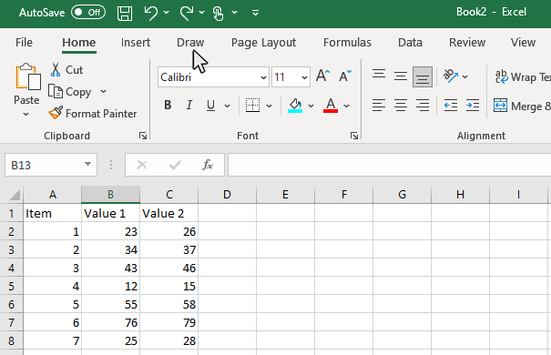
Step 1: Select the Draw Tab on the Ribbon
To activate the highlighter tool, you will first need to select the draw tab on the ribbon. You will then see the Input Mode, Drawing Tools, Convert and Replay panels appear.
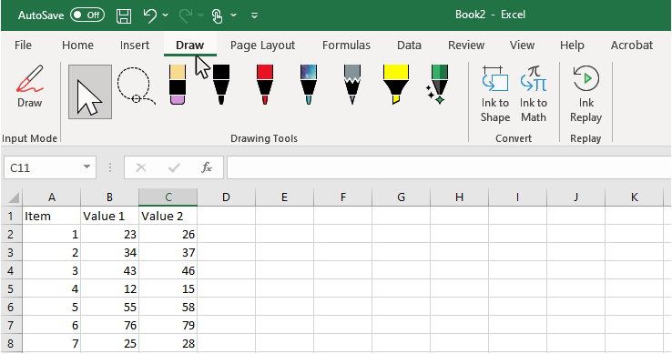
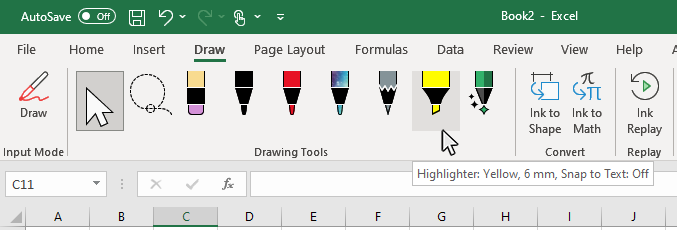
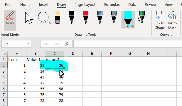
Step 2: Select the Highlighter Brush on the Drawing Tools panel
There are a number of drawing tools on the Drawing tools including the Eraser, Black Pen, Red Pen, Galaxy Pen, Highlighter, and Action Pen. Select the Highlighter
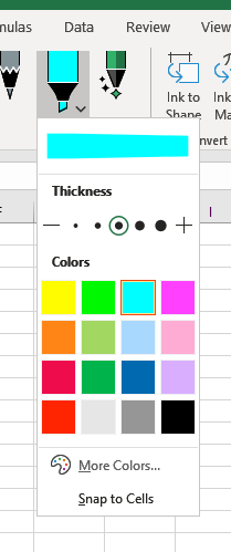
Step 3: Configure the Highlighter color and thickness
Use the cursor to click on a blank area on your chart. Make sure to click on a blank area in the chart. The border around the entire chart will become highlighted. Once you see the border appear around the chart, then you know it is ready to be changed.
Step 4: Highlight the spreadsheet
Use the cursor and click on the area of your spreadsheet that you want to highlight. When you apply the highlighter like this, the brush will work just like a marker on the sheet.
Thanks for checking out this tutorial. If you need additional help, you can check out some of our other free Excel Chart tutorials, or consider taking an Excel class with one of our professional trainers.